This is the second post in a two-part series of posts in which I aim to illustrate a few basic concepts related to Bayesian inference. If you haven't yet, I recommend you check out the first part of the series before going ahead with this one.
In this demo, I will show three sampling techniques that can be used to perform Bayesian inference, using the same toy example introduced in my last write-up.
To re-cap, in my previous post I presented the general ideas behind Bayesian inference and applied them to a 1-D logistic regression problem, regarding the effect of age on Coronary Heart Disease.
Recall that our main goal is to calculate the posterior distribution of our model's parameters given our data and a prior distribution over the parameters:
$$ p(\theta | y) = \dfrac{p(y | \theta) p(\theta)}{\int p(y | \theta) p(\theta) d\theta } $$In general, we also want to calculate quantities e.g. parameter means, quantiles, etc. that can normally be expressed as expectations:
$$ \mathbb{E}[f(\theta)] = \int f(\theta)p(\theta | y)d\theta $$The complications in most examples of Bayesian inference comes from the difficulty in evaluating these integrals.
In Part 1, thanks to the simplicity of our example problem, we were able to explicitly write out the posterior density function and evaluate it on a finite grid of possible parameter values. This allowed us to calculate interesting posterior quantities by performing weighted sums over the grid values. We were also able to generate posterior samples by sampling each grid point with probability proportional to its density value.
However, we noted how this approach would not work well in more complicated cases, which motivates the techniques below.
In most practical cases, we cannot evaluate the posterior density on a grid, due to the difficulties outlined above. Instead, methods based on sampling, also known as Monte Carlo methods, are used.
Basically, if we are able to generate samples $\theta_s$ from the posterior distribution, we can estimate any expectations as follows:
$$ \mathbb{E}[f(\theta)] = \int f(\theta)p(\theta)d\theta \approx \frac{1}{S} \sum_{s=1}^S f(\theta_s) $$The key question is, of course, how to generate samples from $p(\theta | y)$.
We will take a look a two different types of methods:
The basic idea behind importance sampling is to sample from a well-known, "simple" distribution (known as the proposal distribution) and weigh our samples by the ratio between our target and proposal densities in order to calculate expectations.
More formally, this can be expressed as follows:
where $w(\theta) = \frac{p(\theta)}{g(\theta)}$ are the importance weights and $\theta_1, ..., \theta_S$ are sampled from $g(\cdot)$.
Let's implement importance sampling to calculate parameter means in our practical logistic regression example. As proposal distribution, we will use a multivariate (2-D) normal with the following mean and covariance matrix:
The contour plots for the proposal distribution are shown below.
Now, let's draw from this distribution and assign a weight equal to the target-to-proposal density ratio to each sample. The scatter plots below represent the following:
From the scatter plots above, we see that the samples with highest importance resemble the area of highest posterior mass, which we manually computed using grid evaluation on Part 1. It's worth noting that most of the proposal samples have a very small importance weight as they clearly fall very far from the region of interest. Our proposal multivariate normal distribution does not approximate the target distribution very well, which leads to "wasting" many proposal samples.
The histogram of the importance weights' values, shown below, confirms this intuition. In fact, the importance weights are distributed with a fairly high skew. In other words, only a few samples will significantly contribute to the estimates we care about.
It's easy to imagine this method becoming fairly inefficient without the right proposal distribution, especially in high-dimensional settings. Moreover, when the importance weights are heavily skewed, our estimates might not be very reliable, given that only a few samples will significantly contribute to the estimates' values, leading to high variance in our estimates.
We can use the importance-weighted samples to find, for example, the mean & standard deviation of our parameters $\alpha$ and $\beta$, which turn out to be:
These are not too far from the estimates we achieved using grid-evaluation on my previous post.
In many cases, sampling methods like importance sampling are simply not practical. As we have seen, we can spend a lot of our "sampling efforts" in areas of the parameter space that really don't contribute to our estimates, since they are far from the region of high posterior mass.
This motivates a more sophisticated class of methods that generate posterior samples in a sequential manner, trying to explore the parameter space more efficiently. These methods are generally known as Markov chain Monte Carlo (MCMC), given that the sequence of parameter samples constitutes a Markov Chain.
While the details of MCMC are beyond the scope of this small demo, we can take a look at two popular MCMC methods in practice using our logistic regression example, to get an intuition of how MCMC works.
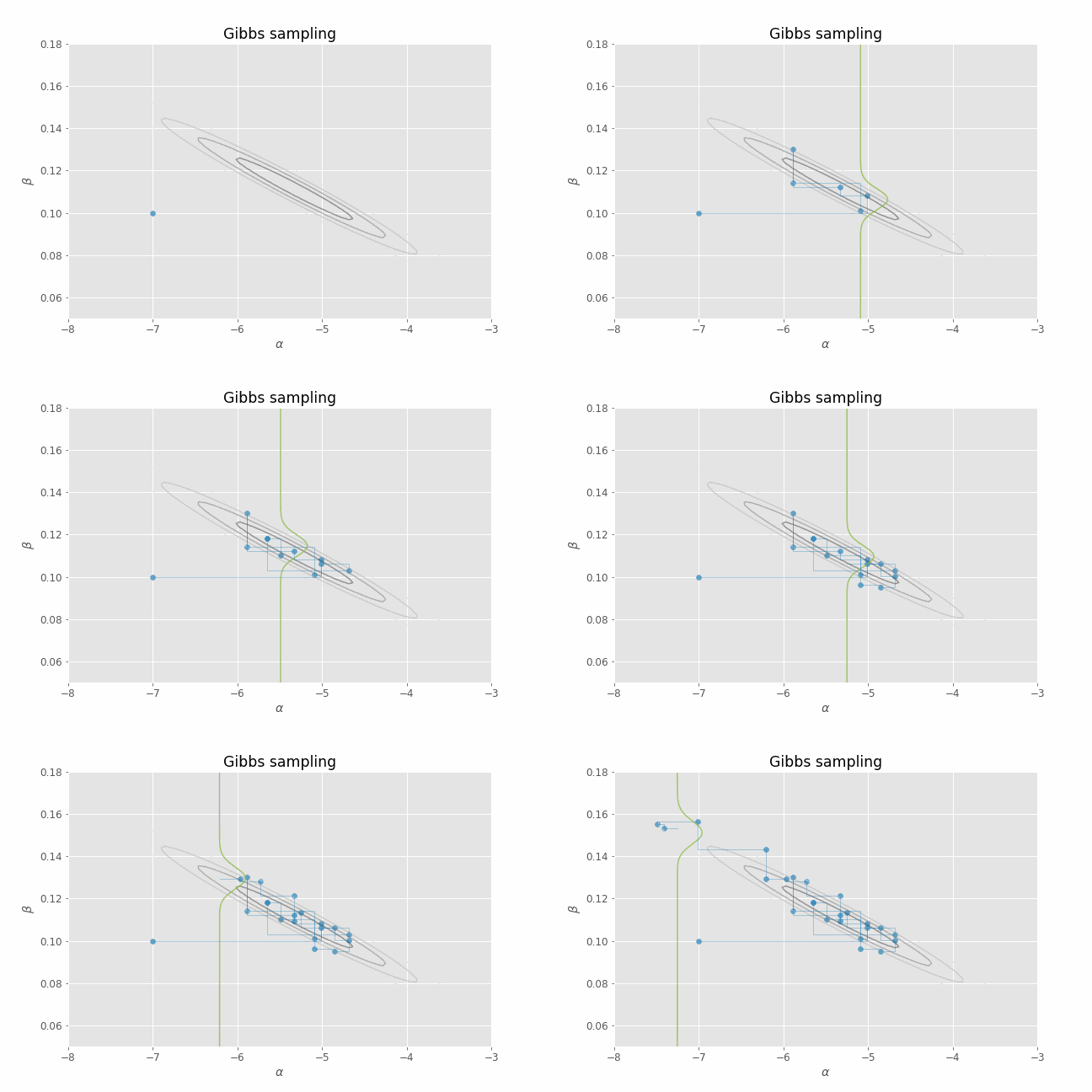
A popular MCMC algorithm is Gibbs sampling. The basic idea behind Gibbs sampling is to iteratively sample from the one-dimensional conditional posteriors. At each iteration of a Gibbs sampling process, we cycle through each dimension in our parameter vector, drawing each parameter conditional on the value of the rest.
More formally, we can express the Gibbs sampling procedure as follows:
where $p(\theta_j | \theta_{-j}^{t-1}, y) = p(\theta_j | \theta_1^t, \theta_2^t, ..., \theta_{j-1}^t, \theta_{j+1}^{t-1}, ..., \theta_d^{t-1}, y)$ is the conditional posterior of the $j$-th parameter at iteration $t$.
The motivation behind Gibbs samping is that it is siginificantly easier to sample from a one-dimensional distribution than from a multi-parameter distribution. In many cases, complex posteriors are built from several conditional distributions that are easy to sample from, which makes Gibbs sampling particularly fitting.
Let's visualize this process in action using our CHD logistic regression example. Several iterations of Gibbs sampling are shown in the animation below. Note that we only need to provide an initial value of the parameters ($\alpha, \beta$) for the algorithm. From that point on, we just alternate between sampling from $p(\alpha | \beta_t, y)$ and $p(\beta | \alpha_t, y)$ for a certain number of iterations. I have added the posterior contour plots to the animation to have a better idea of where the posterior mass lies and to confirm that, indeed, our Gibbs sampler is able to produce parameter samples that cover that region. I have also added a representation of the 1-D conditional density (in green) at each point for illustrative purposes.

Another widely popular MCMC method is the Metropolis algorithm and its generalization, the Metropolis-Hastings algorithm. In a similar way to importance sampling, this method also uses the concept of a proposal distribution. In particular, at each step of the Metropolis algorithm we sample from our proposal distribution (also referred to as jumping distribution), which generally depends on the current iterate, and either accept or reject the proposed sample with probability proportional to the ratio of its posterior density to the previous iterate's posterior density.
More formally, this is the full Metropolis algorithm:
The Metropolis-Hastings algorithm includes a slight modification that allows this algorithm to work when the jumping distribution is not symmetric.
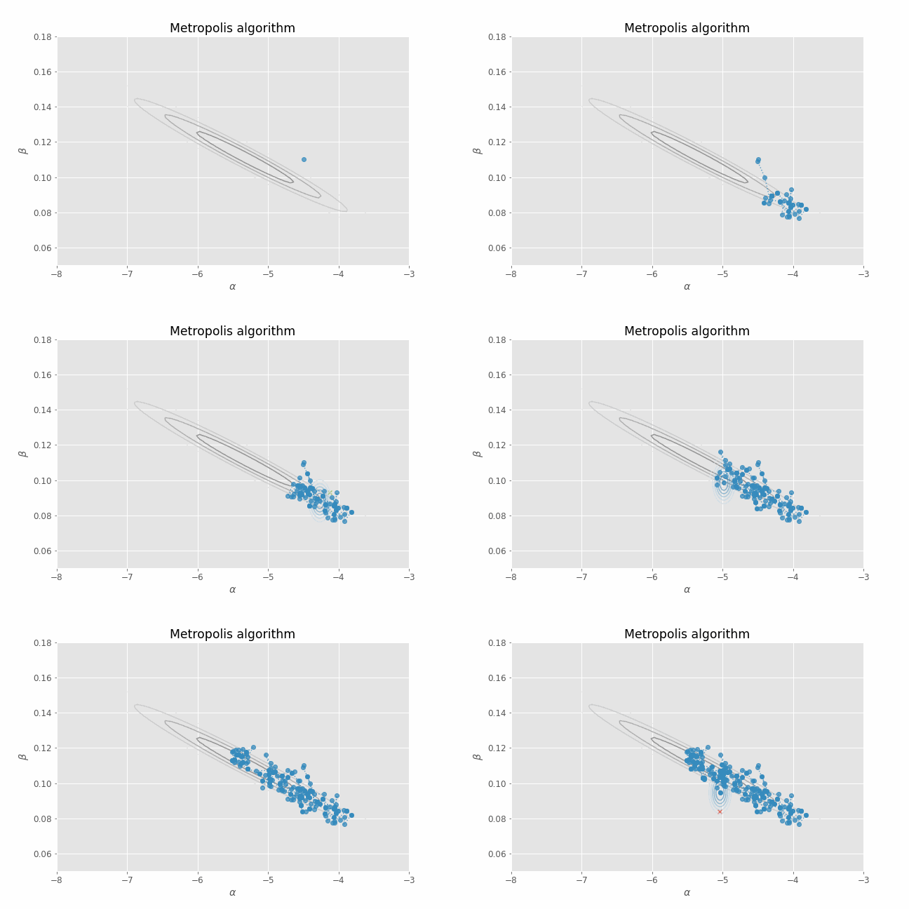
Now let's visualize the Metropolis algorithm in action with our CHD example. At each step, our jumping distribution will be a normal distribution with a fixed covariance matrix and centered at the current value of the parameter sample chain.
The covariance matrix of the proposal distribution is, in a way, a hyperparameter for the algorithm that can roughly be thought of as a "step-size". A small variance will lead to accepting a higher number of our proposed samples but the chain will also require more iterations to explore a bigger region of the parameter space. On the other hand, a big variance will probably lead to more rejected samples but it might allow us to explore bigger regions of parameter space more quickly.
In the animation below, the jumping covariance matrix was:
$$ \Sigma = \begin{bmatrix} 0.01 & 0 \\ 0 & 5.625 \cdot 10^{-5} \end{bmatrix} $$As you can see in the animation below, this Metropolis algorithm run takes some time to explore a significant area where the posterior mass lies. A lot of the proposals are rejected and the algorithm "struggles" to find other regions of the parameters, farther from the initialization point.

To summarize, in this second (and final, for now) post on the basics of Bayesian inference we have seen three methods to generate samples from our posterior distribution:
Hopefully, this helps demystify some of the aspects of sampling techniques in the context of Bayesian inference.
You can check out the code used to generate this report on my GitHub.
Hosmer, D.W., Lemeshow, S. and Sturdivant, R.X. (2013) Applied Logistic Regression, 3rd ed., New York: Wiley
Gelman, A., Carlin, J. B., Stern, H. S., Dunson, D., Vehtari, A. & Rubin, D. B. (2013). Bayesian data analysis (3rd ed). Chapman & Hall/CRC